2.F: STRING & rbioapi

Introduction

STRING is a comprehensive database of known and predicted protein-protein associations. It integrates direct physical interactions and indirect functional associations from experimental evidence, curated databases, text mining, co-expression, and computational predictions. rbioapi provides a consistent R interface to STRING’s mapping, network, homology, annotation, and enrichment API resources.

The `species` argument

Most rbioapi STRING functions accept a species argument containing an NCBI Taxonomy identifier, such as 9606 for human. Supplying it is recommended because it helps STRING resolve ambiguous identifiers.

For the network, interaction-partner, homology, PPI-enrichment, network-image, and enrichment-image functions, species is required when the input contains more than 10 unique IDs. Mapping, functional-enrichment, and functional-annotation requests do not have this local restriction. The limit is based on unique IDs rather than the length of the original vector.

Map your IDs to STRING IDs

Although STRING recognizes a variety of identifiers, mapping them to STRING IDs before using other rbioapi STRING functions makes subsequent requests faster and less ambiguous.

## 1. Create a vector of protein identifiers
proteins <- c(
  "p53", "BRCA1", "cdk2", "Q99835", "CDC42", "CDK1", "KIF23",
  "PLK1", "RAC2", "RACGAP1", "RHOA", "RHOB", "PHF14", "RBM3"
)

## 2. Map the protein identifiers
proteins_mapped_df <- rba_string_map_ids(ids = proteins, species = 9606)


## 3. Use the mapped STRING IDs in the remaining examples
proteins_mapped <- proteins_mapped_df$stringId

Get interaction network of a protein set

You can retrieve interactions among the proteins in your set, together with the scores for each STRING evidence channel. Use required_score to set the minimum interaction score and network_type to select functional or physical associations.

See the Value section of the rba_string_interactions_network() manual for descriptions of the returned columns.

int_net <- rba_string_interactions_network(
  ids = proteins_mapped,
  species = 9606,
  required_score = 500
)

Instead of supplying protein identifiers, you can retrieve the network formed by proteins annotated with a STRING functional term. In this mode, set ids = NULL and supply both network_term_id and species. rba_string_functional_terms() can search for functional terms using either an identifier or descriptive text:

tcr_terms <- rba_string_functional_terms(
  term_text = "T cell receptor signaling pathway",
  species = 9606
)

The first match for this search is GO:0050852, which identifies the GO term “T cell receptor signaling pathway”:

term_net <- rba_string_interactions_network(
  ids = NULL,
  network_term_id = "GO:0050852",
  species = 9606,
  required_score = 900
)

The proteinCount column contains the complete number of proteins annotated with each term, while preferredNames and stringIds are returned as list-columns. The ids and network_term_id input modes cannot be combined.

Get interaction partners of a protein set

The previous example returned interactions among the input proteins. To retrieve proteins that interact with one or more input proteins, including proteins outside the input set, use rba_string_interaction_partners():

## This example uses one protein (CD40), but `ids` can contain multiple proteins
int_partners <- rba_string_interaction_partners(
  ids = "9606.ENSP00000361359",
  species = 9606,
  required_score = 900
)

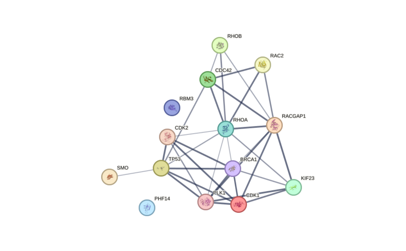
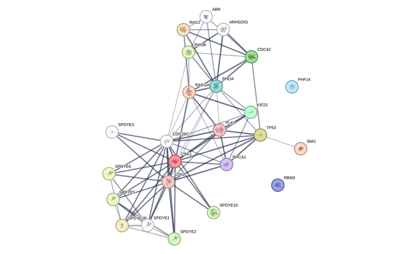
Get network image of a protein set

STRING can render the interaction network as a static image. The rba_string_network_image() function supports several options for controlling the network contents and appearance; see the function manual for details. It also supports the same network_term_id input mode described above.

## Example 1:
graph_ppi1 <- rba_string_network_image(
  ids = proteins_mapped,
  image_format = "image",
  species = 9606,
  save_image = FALSE,
  required_score = 500,
  network_flavor = "confidence"
)

For example, the network for a functional term can be rendered with:

term_image <- rba_string_network_image(
  ids = NULL,
  network_term_id = "GO:0050852",
  species = 9606,
  required_score = 900,
  save_image = FALSE
)

Network images - Example 1

## Example 2:
graph_ppi2 <- rba_string_network_image(
  ids = proteins_mapped,
  image_format = "image",
  species = 9606,
  save_image = FALSE,
  required_score = 500,
  add_color_nodes = 5,
  add_white_nodes = 5,
  network_flavor = "actions"
)

Network images - Example 2

Enrichment analysis using STRING

STRING supports two complementary enrichment analyses: functional enrichment and protein-protein interaction enrichment. See the STRING publication for methodological details.

Functional enrichment

Functional enrichment tests the supplied protein set against annotation resources including Gene Ontology, KEGG pathways, UniProt Keywords, PubMed publications, Pfam domains, InterPro domains, and SMART domains. The results include raw p-values and false discovery rates. See the current STRING API documentation for details.

enriched <- rba_string_enrichment(
  ids = proteins_mapped,
  species = 9606
)

By default, results are split by category into a list of data frames. We can inspect that structure with str():

str(enriched, max.level = 1)
#> List of 14
#>  $ COMPARTMENTS     :'data.frame':   25 obs. of  10 variables:
#>  $ Component        :'data.frame':   17 obs. of  10 variables:
#>  $ DISEASES         :'data.frame':   11 obs. of  10 variables:
#>  $ Function         :'data.frame':   12 obs. of  10 variables:
#>  $ InterPro         :'data.frame':   3 obs. of  10 variables:
#>  $ KEGG             :'data.frame':   45 obs. of  10 variables:
#>  $ Keyword          :'data.frame':   14 obs. of  10 variables:
#>  $ NetworkNeighborAL:'data.frame':   5 obs. of  10 variables:
#>  $ PMID             :'data.frame':   100 obs. of  10 variables:
#>  $ Process          :'data.frame':   148 obs. of  10 variables:
#>  $ RCTM             :'data.frame':   59 obs. of  10 variables:
#>  $ SMART            :'data.frame':   1 obs. of  10 variables:
#>  $ TISSUES          :'data.frame':   12 obs. of  10 variables:
#>  $ WikiPathways     :'data.frame':   46 obs. of  10 variables:

Let us see the “KEGG” results as an example. Below, we can see which terms of the KEGG pathways database were over-represented:

Please Note: Other services supported by rbioapi also provide Over-representation analysis tools. Please see the vignette article Do with rbioapi: Over-Representation (Enrichment) Analysis in R (link to the documentation site) for an in-depth review.

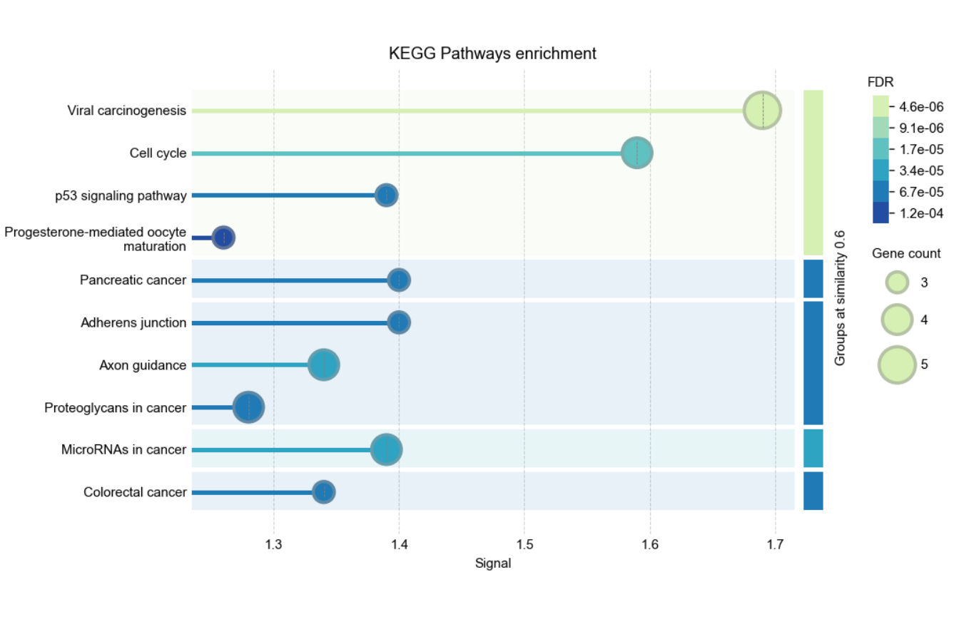
Functional enrichment plot

The enrichment-figure endpoint summarizes one enrichment category as a plot. Use rba_string_enrichment_image() to control the category, grouping, palette, ranking variable, output format, and number of displayed terms. This example visualizes the KEGG enrichment for the same protein set:

graph_enrich <- rba_string_enrichment_image(
  ids = proteins_mapped,
  species = 9606,
  category = "KEGG",
  image_format = "image",
  save_image = FALSE,
  group_by_similarity = 0.6
)

Visualization of enrichment analysis results

Protein-protein interaction enrichment

PPI enrichment tests whether the input network contains more interactions than expected for a similarly sized protein set drawn from the background proteome. It can therefore identify evidence of functional relatedness without relying on annotation enrichment.

rba_string_enrichment_ppi(
  ids = proteins_mapped,
  species = 9606
)
#> $number_of_nodes
#> [1] 14
#> 
#> $number_of_edges
#> [1] 40
#> 
#> $average_node_degree
#> [1] 5.71
#> 
#> $local_clustering_coefficient
#> [1] 0.694
#> 
#> $expected_number_of_edges
#> [1] 19
#> 
#> $p_value
#> [1] 1.35e-05

Get functional annotations

STRING maps proteins to multiple annotation resources. Use rba_string_annotations() to retrieve all annotations assigned to the input proteins rather than only the subset returned by enrichment analysis. PubMed annotations are excluded by default because they can make the response very large.

annotations <- rba_string_annotations(
  ids = "9606.ENSP00000269305",
  species = 9606
)

## Annotation responses can be large, so the result is not shown here

Set allow_pubmed = TRUE to include PubMed annotations with the other categories, or set only_pubmed = TRUE to retrieve only PubMed annotations. only_pubmed takes precedence if both arguments are TRUE.

pubmed_annotations <- rba_string_annotations(
  ids = "9606.ENSP00000269305",
  species = 9606,
  only_pubmed = TRUE
)

How to cite

To cite STRING (Please see https://string-db.org/cgi/about?footer_active_subpage=references):

Damian Szklarczyk, Rebecca Kirsch, Mikaela Koutrouli, Katerina Nastou, Farrokh Mehryary, Radja Hachilif, Annika L Gable, Tao Fang, Nadezhda T Doncheva, Sampo Pyysalo, Peer Bork, Lars J Jensen, Christian von Mering, The STRING database in 2023: protein–protein association networks and functional enrichment analyses for any sequenced genome of interest, Nucleic Acids Research, Volume 51, Issue D1, 6 January 2023, Pages D638–D646, https://doi.org/10.1093/nar/gkac1000

To cite rbioapi:

Moosa Rezwani, Ali Akbar Pourfathollah, Farshid Noorbakhsh, rbioapi: user-friendly R interface to biologic web services’ API, Bioinformatics, Volume 38, Issue 10, 15 May 2022, Pages 2952–2953, https://doi.org/10.1093/bioinformatics/btac172

Session info

#> R version 4.6.1 (2026-06-24)
#> Platform: x86_64-pc-linux-gnu
#> Running under: Ubuntu 24.04.4 LTS
#> 
#> Matrix products: default
#> BLAS:   /usr/lib/x86_64-linux-gnu/openblas-pthread/libblas.so.3 
#> LAPACK: /usr/lib/x86_64-linux-gnu/openblas-pthread/libopenblasp-r0.3.26.so;  LAPACK version 3.12.0
#> 
#> locale:
#>  [1] LC_CTYPE=C.UTF-8       LC_NUMERIC=C           LC_TIME=C.UTF-8       
#>  [4] LC_COLLATE=C.UTF-8     LC_MONETARY=C.UTF-8    LC_MESSAGES=C.UTF-8   
#>  [7] LC_PAPER=C.UTF-8       LC_NAME=C              LC_ADDRESS=C          
#> [10] LC_TELEPHONE=C         LC_MEASUREMENT=C.UTF-8 LC_IDENTIFICATION=C   
#> 
#> time zone: UTC
#> tzcode source: system (glibc)
#> 
#> attached base packages:
#> [1] stats     graphics  grDevices utils     datasets  methods   base     
#> 
#> other attached packages:
#> [1] rbioapi_0.8.3
#> 
#> loaded via a namespace (and not attached):
#>  [1] httr_1.4.8        cli_3.6.6         knitr_1.51        rlang_1.3.0      
#>  [5] xfun_0.60         otel_0.2.0        png_0.1-9         textshaping_1.0.5
#>  [9] jsonlite_2.0.0    DT_0.34.0         htmltools_0.5.9   ragg_1.5.2       
#> [13] sass_0.4.10       rmarkdown_2.31    grid_4.6.1        crosstalk_1.2.2  
#> [17] evaluate_1.0.5    jquerylib_0.1.4   fastmap_1.2.0     yaml_2.3.12      
#> [21] lifecycle_1.0.5   compiler_4.6.1    fs_2.1.0          htmlwidgets_1.6.4
#> [25] systemfonts_1.3.2 digest_0.6.39     R6_2.6.1          curl_7.1.0       
#> [29] magrittr_2.0.5    bslib_0.11.0      tools_4.6.1       pkgdown_2.2.1    
#> [33] cachem_1.1.0      desc_1.4.3

Moosa Rezwani

2026-07-30

Introduction

The `species` argument

Map your IDs to STRING IDs

Get interaction network of a protein set

Get interaction partners of a protein set

Get network image of a protein set

Enrichment analysis using STRING

Functional enrichment

Functional enrichment plot

Protein-protein interaction enrichment

Get functional annotations

See also in Functions’ manuals

How to cite

Links

Session info

2.F: STRING & rbioapi

Moosa Rezwani

2026-07-30

Introduction

The species argument

Map your IDs to STRING IDs

Get interaction network of a protein set

Get interaction partners of a protein set

Get network image of a protein set

Enrichment analysis using STRING

Functional enrichment

Functional enrichment plot

Protein-protein interaction enrichment

Get functional annotations

See also in Functions’ manuals

How to cite

Links

Session info

The `species` argument